Machine Learning | Multiple Linear Regression

Multiple linear regression is a statistical technique used in machine learning to model the relationship between one dependent variable and two or more independent variables. It extends the concept of simple linear regression by incorporating multiple predictors. This method is widely used for prediction and forecasting in various fields such as economics, finance, and the social sciences, where understanding the impact of several factors on a single outcome is crucial.

In the last post we learnt about Linear regression with one variable. The hypothesis function for it was:

ℎ_ \theta(x) = \theta_ 0 + \theta_ 1 x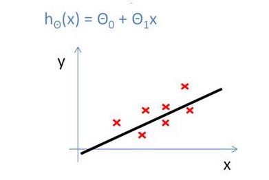

What if, we have more than one independent variables or features. Then our hypothesis function could be like:
h_ \theta (x) = \theta_ 0 + \theta_ 1 x_1 + \theta_ 2 x_2 + \theta_ 3 x_3

And our (y vs x plots) graphs would be like:

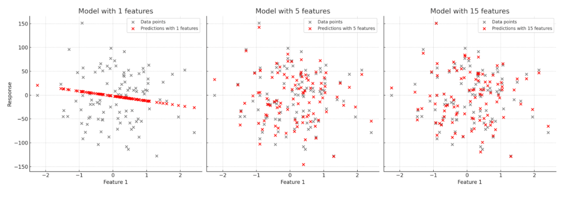
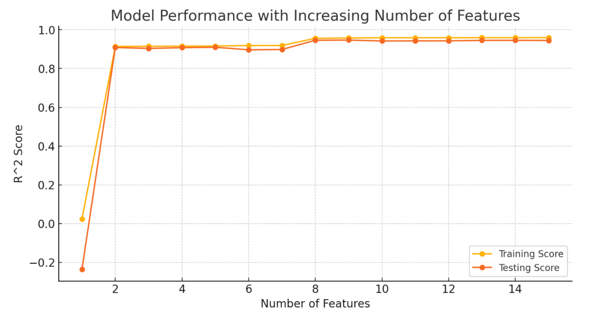
As we could see, with more independent variables, our model exactly fits the training data. However, if a model uses too many independent variables or learns the noise in the training data too well, it can lead to what we call Overfitting. This means that while the model fits the training data perfectly, it performs poorly on new, unseen data because it hasn’t generalized well.

Overfitting occurs when a model becomes too complex by using too many independent variables, fitting the training data too closely and capturing noise. This results in poor performance on test data.

On the other hand, if our model is too simple and doesn’t use enough features, it won’t capture the underlying patterns in the data, leading to Underfitting. This means the model performs poorly both on the training data and on new data.

Underfitting occurs when a model is too simple to capture the underlying patterns in the data, leading to poor performance on both the training data and test data. This usually happens when there are too few independent variables or the model is not sufficiently flexible.

Now while underfitting would result in wrong predictions, overfitting is also not good for our machine learning model. Because though, it would match the training set well, it might not work well with the test or actual data. As it is biased towards our training set and will only works well with the same or similar input. It would give poor performance on variable data sets.

How to choose the number of parameters?

For a good machine learning model, it is crucial to achieve a balance between underfitting and overfitting. While underfitting can be addressed by introducing more features, solving overfitting requires more careful strategies. So, how do we solve overfitting?

To avoid overfitting:

1. One natural way is to reduce the number of parameters and adjust them so that it doesn’t just works well with the given set of data. This involves simplifying the model by removing less important features, ensuring that it doesn’t just work well with the training data but generalizes better to new or test data.
2. Second way is Regularisation. It means to reduce the magnitude (effect) of certain parameters \theta_ i while keeping all the features. In general, Regularisation adds a penalty term to the cost function that discourages the model from fitting the noise in the training data.

Regularisation

Regularisation helps prevent overfitting by adding a penalty term to the cost function, which discourages the model from becoming too complex. By understanding and applying regularisation techniques, you can build models that generalize well to new data.

For instance, if our hypothesis function is:

h_ \theta (x) = \theta_ 0 + \theta_ 1 x_1 + \theta_ 2 x_2 + \theta_ 3 x_3 + ….

and we penalise \theta_ 3 and remaining terms in the cost function. Then, our cost function will become like (first part is the mean squared error, and the second part is the regularisation term):

J( \theta ) = 1/2m[\sum_{i=1}^{m} ({h_ \theta (x^i)} - {y^i})^{2} + \lambda \sum_{j=3}^{n} (\theta_ j)]

(L1 Regularisation (Lasso) adds the absolute value of the coefficients as a penalty term to the cost function)

J( \theta ) = 1/2m[\sum_{i=1}^{m} ({h_ \theta (x^i)} - {y^i})^{2} + \lambda \sum_{j=3}^{n} (\theta_ j ^2)]

(L2 Regularisation (Ridge) adds the square of the coefficients as a penalty term to the cost function)

Here, \lambda \sum_{j=3}^{n} (\theta_ j) and \lambda \sum_{j=3}^{n} (\theta_ j ^2) are the regularisation terms and \lambda is the regularisation parameter that controls the penalty’s strength. Regularisation keeps model coefficients small, reducing overfitting and improving generalization.

Remember, our goal is to minimise cost function. Now, by introducing regularisation we are increasing the value of cost function for certain parameters (\theta_ j)s . This penalty discourages overfitting by reducing the magnitude (or effect) of the selected parameters (\theta_ j)s  on model’s performance.

Choosing Regularisation factor (\lambda )

Selecting the appropriate value for the regularisation factor \lambda is crucial for balancing bias and variance in your model.

• If \lambda is too large, it may cause underfitting.
• And if \lambda is too small, it may have no effect.

To prevent overfitting, we need to choose the regularisation factor according to our data. This involves systematically trying different values and observing their impact on the model’s performance. By using a trial and error approach, we can identify the value of \lambda that optimizes the balance between making the model complex enough to capture the patterns in the data, but not so complex that it starts to capture noise and overfit.

By systematically evaluating \lambda and using trial and error, you can choose a value that optimizes model and prevents overfitting, improving the model’s performance on new unseen data.

Understanding and applying these practices, you can build robust ML models that generalizes well on different data sets. Balancing model complexity and using techniques like regularisation, you can create models that are not only accurate but also perform well across diverse use-cases.

Reference:
Coursera | Online Courses & Credentials From Top Educators. Join for Free | Coursera